11. R-Squared#
R-squared is a regression metric. It has the following formula:
Where \(RSS\) is the sum of squared residuals and \(TSS\) is the total sum of squares.
In other words, \(RSS\) is the total squared difference between the target values \(y\) and the predictions \(y_i\). Mathematically, this is:
\(TSS\) is the total difference between \(y\) and the mean of \(y\) which we denote as \(\bar{y}\). Mathematically, this is:
The quotient in the \(R^2\) formula compares our model with a baseline that is just the mean of \(y\). If our model is better at predicting \(y\) than the mean \(\bar{y}\), then \(RSS\) will be smaller than \(TSS\) and therefore the quotient \(\frac{RSS}{TSS}\) will be less than 1.
If the model is not better at predicting \(y\) than the mean \(\bar{y}\), then \(TSS\) will be smaller than \(RSS\) and \(\frac{RSS}{TSS}\) will be greater than 1.
Why in the \(R^2\) formula do we take \(\frac{RSS}{TSS}\) from 1? It makes it easier to interpret. If our model outperforms the mean \(\bar{y}\) then \(R^2\) will be between 0 and 1. The closer the 1 the better. If our model is not better than the mean \(\bar{y}\) then \(R^2\) will be less than 0.
12. Example 1: Linear Target#
Suppose we have data that is generated from the following underlying process:
Where \(\epsilon\) is a noise term. Let us model it with a simple linear regression model. Create the data and fit the model.
import numpy as np
import matplotlib.pyplot as plt
from sklearn.linear_model import LinearRegression

n = 100
x = np.random.normal(0, 1, n).reshape(-1, 1)
epsilon = np.random.normal(0, 0.1, n).reshape(-1, 1)
y = 0.5 * x + 1 + epsilon

model = LinearRegression()
model.fit(x, y)
y_hat = model.predict(x)

fig, ax = plt.subplots()
ax.scatter(x[:, 0], y, label="Original data", color="tab:blue")
ax.plot(x[:, 0], y_hat, label="Predictions", color="tab:orange")
ax.legend();
---------------------------------------------------------------------------
ModuleNotFoundError                       Traceback (most recent call last)
Cell In[1], line 1
----> 1 import numpy as np
      2 import matplotlib.pyplot as plt
      3 from sklearn.linear_model import LinearRegression

ModuleNotFoundError: No module named 'numpy'
Create a function for computing \(R^2\).
def r_squared(y_true, y_pred):
    rss = ((y_true - y_pred) ** 2).sum()
    tss = ((y_true - y_true.mean()) ** 2).sum()
    return 1 - rss / tss
Compute the \(R^2\) score for our model’s predictions.
r_squared(y, y_hat)
0.9661874237889019
The \(R^2\) is close to 1 to our model is very good.
12.1. R Squared On Small Datasets Can Give Strange Results#
\(R^2\) compares the model predictions with the mean of the target variable. For small datasets, this mean may not reflect that of the underlying probability distribution.
For example suppose we model a cubic function.
n = 100
x = np.linspace(-1.5, 1.5, 100).reshape(-1, 1)
x = np.sort(x)
epsilon = np.random.normal(0, 0.1, n).reshape(-1, 1)
y = x ** 3 + epsilon

model = LinearRegression()
model.fit(x, y)
y_hat = model.predict(x)

fig, ax = plt.subplots()
ax.scatter(x[:, 0], y, label="Original data", color="tab:blue", alpha=0.5)
ax.plot(x[:, 0], y_hat, label="Predictions", color="tab:orange")
ax.legend()
ax.grid(linestyle=":")
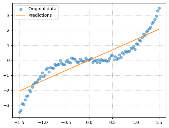
Even though we have modelled our cubic function with a straight line, it is not a bad approximation. Calculate the \(R^2\) for our predictions.
r_squared(y, y_hat)
0.827909114372573
The model fit is quite good. However, if we choose a very small specific subset of the training data, we can get an extrememly negative \(R^2\) value.
mask = (x > 0.5) & (x < 0.7)
x_test = x[mask].reshape((-1, 1))
y_test = y[mask]
y_test_pred = model.predict(x_test)

r_squared(y_test, y_test_pred)
-214.9338556085192
Plot these data points and their mean.
y_test_mean = y_test.mean()

fig, ax = plt.subplots()
ax.scatter(x[:, 0], y, label="Original data", color="tab:blue", alpha=0.5)
ax.plot(x[:, 0], y_hat, label="Predictions", color="tab:orange")
ax.scatter(x_test[:, 0], y_test, label="Test set", color="black")
ax.axhline(y_test_mean, color="gray", linestyle="--", label="Mean of test set")

ax.legend()
ax.grid(linestyle=":")
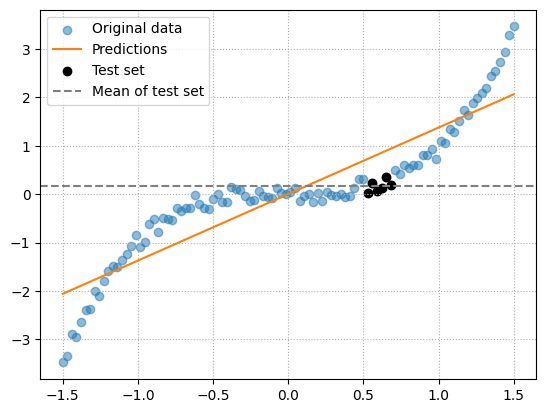
For this small subset of data points, the mean is a better approximation than our model. So, according to \(R^2\), our model is terrible.
This is an unrealistic example but suppose you are predicting house prices in the UK. Suppose you want to see how well your model performs in a certain post code which contains 30 houses. The mean house price for that post code is probably going to be a good approximate and maybe better than a model trained on prices from the whole of the UK which will lead to negative \(R^2\).
If you are using \(R^2\) on a small subset of your entire population you should be aware that your \(R^2\) may be extremely negative if your subset is not representative of your whole population.