9. Linear Regression

Suppose we have a dependent variable \(y\) and dependent variables \(x = (x_1, x_2, \dots, x_n)\). The general form for a linear regression models that predicts the dependent variable is,

\[ f(x) = b + w_1 x_1 + w_2 x_2 + \dots + w_n x_n. \]

Where \(b\) is a bias term. Let us convert these term into matrices and vectors. Suppose we make \(m\) observations so we have \(m\) dependection variables,

\[\begin{split} Y = \begin{bmatrix} y_1 \\ y_2 \\ \vdots \\ y_m \end{bmatrix} \end{split}\]

And \(m\) dependent variables each comprised of \(n\) features,

\[\begin{split} X = \begin{bmatrix} 1 && x_{11} && x_{12} && \dots && x_{1n} \\ 1 && x_{21} && x_{22} && \dots && x_{2n} \\ \vdots && \vdots && \vdots && \dots && \vdots \\ 1 && x_{m1} && x_{m2} && \dots && x_{mn} \\ \end{bmatrix} \end{split}\]

The column of ones is included for the bias term \(b\). We want to find a weight vector,

\[\begin{split} W = \begin{bmatrix} b \\ w_1 \\ w_2 \\ \vdots \\ w_m \end{bmatrix} \end{split}\]

Such that our predictions \(\hat{Y} = X W\) are as close to \(Y\) as possible.

We find such a \(W\) using the pseudoinverse.

\[\begin{split} \begin{align} Y & = X W \\ Y & = X^T X W \\ X^T Y & = X^T X W \\ (X^T X) ^ {-1} X^T Y & = (X^T X) ^ {-1} X^T X W \\ (X^T X) ^ {-1} X^T Y & = W \\ \end{align} \end{split}\]

the matrix \((X^T X) ^ {-1} X^T\) is called the psuedoinverse.

10. Simple Linear Example

Suppose we are trying to model a linear function.

import numpy as np
import matplotlib.pyplot as plt

m = 10
X = np.vstack((np.ones(m), np.linspace(0, 1, m))).T
Y = 2 * X[:, 1] + 1 + np.random.normal(scale=0.2, size=(m))

plt.scatter(X[:, 1], Y, marker="o")

---------------------------------------------------------------------------
ModuleNotFoundError                       Traceback (most recent call last)
Cell In[1], line 1
----> 1 import numpy as np
      2 import matplotlib.pyplot as plt
      4 m = 10

ModuleNotFoundError: No module named 'numpy'

Now we have our data, let us write out model.

class LinearRegression:
    def __init__(self):
        self.W = None

    def fit(self, X, Y):
        self.W = np.linalg.inv(X.T @ X) @ X.T @ Y

    def predict(self, X):
        return X @ self.W

model = LinearRegression()
model.fit(X, Y)
Y_hat = model.predict(X)

plt.scatter(X[:, 1], Y, marker="o")
plt.plot(X[:, 1], Y_hat, color="tab:orange", label="Y_hat")
plt.legend()

<matplotlib.legend.Legend at 0x7ff90fcdf510>

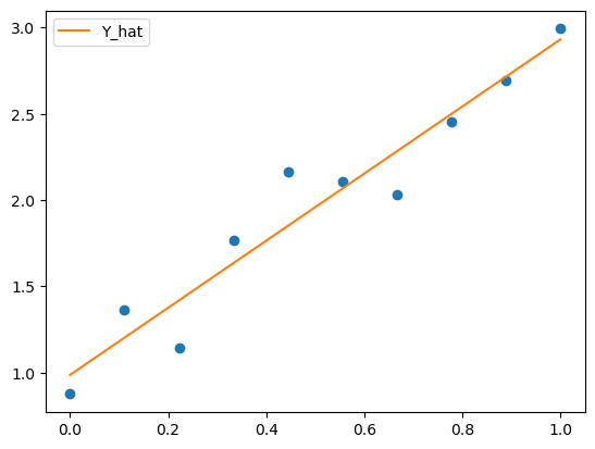
If we look at the parameters of the model, we should find they are similar to the parameters we used to generate the data.

model.W

array([0.98689721, 1.94516279])

The first number is the intercept which was 1 and the second number is the gradient which was 2.

10.1. Fitting our model to a more complicated function

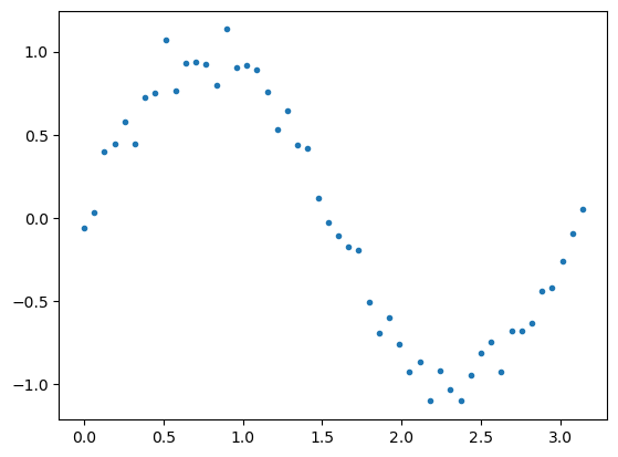
Now let us fit the linear regression model to a sine function

m = 50
x = np.linspace(0, np.pi, m)
X = np.vstack((
    np.ones(m),
    x,
)).T
Y = np.sin(2 * x) + np.random.normal(scale=0.1, size=m)

plt.scatter(x, Y, marker='.')

<matplotlib.collections.PathCollection at 0x7ff90f70e610>

model.fit(X, Y)
Y_hat = model.predict(X)

plt.scatter(x, Y, marker='.')
plt.plot(x, Y_hat, color='tab:orange')

[<matplotlib.lines.Line2D at 0x7ff90f5c52d0>]

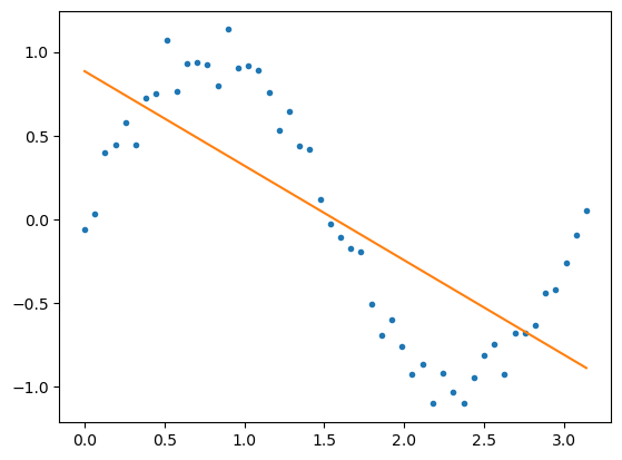
Our models prediction is quite poor. We can try and improve it by adding higher power terms to the model.

for i in range(2, 5):
    X = np.stack([x ** p for p in range(i)]).T
    model.fit(X, Y)
    Y_hat = model.predict(X)
    plt.plot(x, Y_hat, label=f"Degree {i}")

plt.scatter(x, Y, marker='.', color='tab:olive')
plt.legend()

<matplotlib.legend.Legend at 0x7ff90ec6d990>

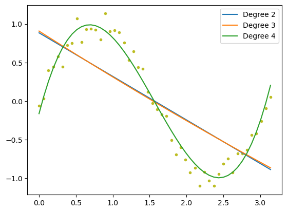
The degree 4 model performs the best.

10.2. Gradient Descent

In the previous section we looked at finding an analytic solutions for the weights, \(W\), of the model. Now we look at gradient descent which the weights by iteratively improving the guess for the weights.

It does this by using a loss function, in this case mean squared error, that gives us a measure of how good the prediction is.

\[ \text{MSE} = \frac{1}{m} \sum_{i=1}^{m}(\hat{y}_i - y_i)^2. \]

Or equally

\[\begin{split} \begin{align} \text{MSE} = & \frac{1}{m} \sum_{i=1}^{m}(X_i W - y_i)^2 \\ = & \frac{1}{m} \sum_{i=1}^{m}\left(\sum_{j=1}^{m}x_{ij}w_j - y_i\right)^2 \\ \end{align} \end{split}\]

We can then find the gradient of the mean squared error with respect to each weight \(w_j\). We find the gradient using the chain rule.

\[\begin{split} \begin{align} \frac{\partial \text{MSE}}{\partial w_k} = & \frac{1}{m} \sum_i x_{ij} \left(\sum_j x_{ij} w_j - y_i\right) \\ = & \frac{1}{m} \sum_i x_{ik} \left(X_i W - y_i\right) \\ = & \frac{1}{m} \sum_i x_{ik} X_i W - \frac{1}{m} \sum_i x_{ik} y_i \\ = & \frac{1}{m} (X_{,k} X W - X_{,k} Y) \end{align} \end{split}\]

Now let us implement this.

class GradientDescent():
    def __init__(self, n_iter=500, learning_rate=0.01):
        self.n_iter = n_iter
        self.W = None
        self.W_hist = None
        self.loss_hist = None
        self.learning_rate = learning_rate

    def fit(self, X, Y):
        m, n = X.shape
        self.W = np.random.normal(size=n)
        self.loss_hist = np.zeros(self.n_iter)
        self.W_hist = np.zeros((self.n_iter, n))

        for i in range(self.n_iter):
            loss = np.mean((X @ self.W - Y) ** 2)
            grad = (2 / m) * (X.T @ X @ self.W - X.T @ Y)
            self.W -= self.learning_rate * grad

            self.loss_hist[i] = loss
            self.W_hist[i] = self.W

    def predict(self, X):
        return X @ self.W

m = 10
x = np.linspace(-1, 1, m)
X = np.vstack((
    np.ones(m),
    x,
)).T

Y = 1 * x + 1 + np.random.normal(scale=0.2, size=(m))

model = GradientDescent()
model.fit(X, Y)
Y_hat = model.predict(X)

fig, ax = plt.subplots(1, 2, figsize=(12, 4))
ax[0].scatter(x, Y)
ax[0].plot(x, Y_hat, color="tab:orange")
ax[1].plot(model.loss_hist)

ax[1].set_ylabel("MSE")
ax[1].set_xlabel("Iteration")

Text(0.5, 0, 'Iteration')

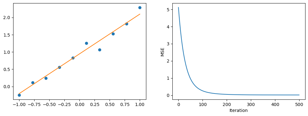
On the left we have the fit of the model and on the right we have the loss curve.