12. Broadcasting in Numpy#

import numpy as np

import os
import pathlib

root = pathlib.Path(os.getcwd())

---------------------------------------------------------------------------
ModuleNotFoundError                       Traceback (most recent call last)
Cell In[1], line 1
----> 1 import numpy as np
      3 import os
      4 import pathlib

ModuleNotFoundError: No module named 'numpy'

12.1. Taking the mean from each row#

If mean have a matrix of shape (2, 3). Using numpy.mean, we can get the mean of each row as a vector with shape (2). In number, we cannot take the vector from the matrix as the shapes are not broadcastable. Numpy checks it two arrays are broadcastable by looking from the right-most dimension to the left. The arrays are broadcastable if:

The dimensions are equal, or
One of the dimensions is 1.

In our example, the array and vector are not broadastable since the right-most dimensions, 3 and 2, are not broadcastable. We can make the arrays broadcastable by adding a dimension to the vector on the right. This means the matrix has shape (2, 3) and the vector has shape (2, 1): 2 is broadcastable to 2 and 3 is broadcastable to 1.

x = np.array([
    [1, 0, -1],
    [3, 2, 1]
])

mean = x.mean(axis=1)  # Array with shape (3,)
try:
    x - mean
except ValueError as e:
    print(e)

mean = mean[:, None]  # Array with shape (2, 1) 

print(x - mean)

operands could not be broadcast together with shapes (2,3) (2,) 
[[ 1.  0. -1.]
 [ 1.  0. -1.]]

12.2. Taking the mean from each column#

In this case, if we find the mean of column and store then in a vector with shape (3,), this is broadcastable with original array since the right most dimensions are the same.

What about the first dimension?

If there are not the same number of dimensions, you can think of numpy filling the missing dimensions with ones.

x = np.array([
    [1, 0, -1],
    [3, 2, 1]
])

mean = x.mean(axis=0)  # Array with shape (2,)
print(x - mean, end="\n\n")

mean = mean[None, :]
print(x - mean)

[[-1. -1. -1.]
 [ 1.  1.  1.]]

[[-1. -1. -1.]
 [ 1.  1.  1.]]

12.3. Example from one point to every other point#

Suppose we want to find the euclidean distance from one point to every other point.

x = np.array([1.0, 1.0])

y = np.array([
    [1.0, 1.0],
    [1.0, 2.0],
    [0.0, 0.0],
])

((x[None, :] - y) ** 2).sum(axis=1) ** (0.5)

array([0.        , 1.        , 1.41421356])

How to we work out the distance from every point in \(y\) to every other point in \(y\)? The non-trivial part is the substraction, this is where we take advantage of broadcasting. The solution is,

\[ \begin{align} y[3 \times 1 \times 2] - y[1 \times 3 \times 2]. \end{align} \]

Why does this work? The final shape will be (3, 3, 2) which is what we want. To make it so the arrays can be taken away from one another. Think of the dimensions where the shape is 1 being stretched to match the other matrix. So the second dimension for the array on the left is stretched to have shape 3.

What is put in the extra entries? The elements in the dimensions right of the one we are stretching are essentially copied. So, for the array on the left, since the second dimension is being stretched, the third dimension will be copied to fill in the gaps.

(y[:, None, :] - y[None, :, :])

array([[[ 0.,  0.],
        [ 0., -1.],
        [ 1.,  1.]],

       [[ 0.,  1.],
        [ 0.,  0.],
        [ 1.,  2.]],

       [[-1., -1.],
        [-1., -2.],
        [ 0.,  0.]]])

So the left matrix contains three (3, 2) matrix that only contain copies of one of the rows. The matrix on the right has the original (3, 2) matrix copied three times.

Let us now calculate all the distances.

((y[:, None, :] - y[None, :, :]) ** 2).sum(axis=2) ** (0.5)

array([[0.        , 1.        , 1.41421356],
       [1.        , 0.        , 2.23606798],
       [1.41421356, 2.23606798, 0.        ]])

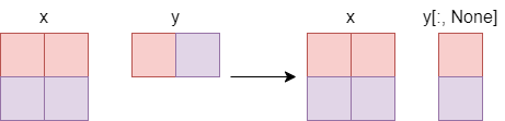
12.4. Visual example#

Here the goal is to end up with a matrix of zeros. Here is simple 2D example.

x = np.array([
    [1, 1],
    [2, 2],
])

y = np.array([1, 2])

x - y[:, None]

array([[0, 0],
       [0, 0]])

Below is a visual representation of what is going on here. It is easy to see here what happend when the y[:, None] is stretched.

import IPython
IPython.display.Image(root / "Images" / "2d_example.png")

../_images/277ee75ed0594d6af8ce43a8bd608731243f0352add0bc4437178567ed12dd7b.png

Lets us look at a more complicated 3d example.

x = np.array([
    [[1, 2],
     [1, 2],
     [1, 2]],
    [[1, 2],
     [1, 2],
     [1, 2]],
])

y = np.array([1, 2])
x - y[None, None, :]

array([[[0, 0],
        [0, 0],
        [0, 0]],

       [[0, 0],
        [0, 0],
        [0, 0]]])